Image similarity measures play an important role in image fusion algorithms and applications, such as duplicate product detection, image clustering, visual search, change detection, quality evaluation, and recommendation tasks. These measures essentially quantify the degree of visual and semantic similarity of a pair of images. In other words, they compare two images and return a value that tells you how visually similar they are.
The input images may be a set of images obtained from the same scene or object taken from different environmental conditions, angles, lighting conditions, or edited transformations of the same image. In most use cases, the degree of similarity between the images is very important. In other use cases, the aim is to consider whether two images belong to the same category.
To perform image similarity, we need to consider two elements. First, we find the set of features that can be used to describe the image content and, second, we apply a suitable metric to assess the similarity of two images based on the feature space. An image's feature space can be for the entire image or just for a small group of pixels within the image, such as regions or objects.
The resulting measure can be different depending on the types of features. Typically, the feature space is assumed to be Euclidean. Euclidean is a space in any finite number of dimensions (originally three-dimensional), in which points are defined by coordinates (one for each dimension) and the distance between two points is calculated by a distance formula. Generally, algorithms that are used to assess the similarity between two images aim to reduce the semantic gap between low-level features and high-level semantics as much as possible.
Depending on the use case, there may be algorithms that can be used for measuring similarity. However, in most cases, evaluating the math for a metric and ensuring the correct implementation for your use case is a challenge. This post introduces a Python package, developed by UP42, that has several ready-to-use algorithms for applying similarity measures.
We used this package to evaluate a final image's quality in the analysis outlined in our recent publication. After doing an inference on the image, we used image similarity measures to compare it with the ground truth image and check whether the predicted image kept the ground truth's essential features.
How To Use Our Python Package
Similarity measure algorithms can usually be implemented by checking the formula and implementing it in your preferred coding language. However, having several options available can help remove the effort and frustration behind understanding every formula in metric. To help with this, we've developed a Python package with eight image similarity metrics that can be for either 8-bit (visual) or 12-bit (non-visual) images. You can use this package either via the command line (CLI) or by importing it directly into your Python code, as long as you are running Python version 3.6, 3.7, or 3.8.
Here is an example of using the package via the CLI:
image-similarity-measures --org_img_path=path_to_first_img
--pred_img_path=path_to_second_img --mode=tif
--org_img_path_ indicates the path to the original image, and pred_img_path indicates a path to the predicted or disordered image, which is created from the original image. --mode is the image format with the default set to tif. Other options are png or jpg. --write_to_file can be used to write the final result to a file. You can set it to false if you don't want a final file. Finally, --metric is the name of the evaluation metric that, by default, is set to psnr. However, it can also be on the following:
rmsessimfsimissmsresamuiq
If you want to use it in your Python code, you can do so as follows:
import cv2
import image_similarity_measures
from image_similarity_measures.quality_metrics import rmse, psnr

in_img1 = cv2.imread('img1.png')
in_img2 = cv2.imread('img2.png')

out_rmse = rmse(in_img1, in_img2)
out_psnr = psnr(in_img1, in_img2)
You can check out the repository in Github to get more information, review the code, or even contribute to the Open Source project yourself!
The Eight Similarity Measures, Explained
We have implemented eight different metrics in our python package. Each of these metrics has distinct benefits and tells you something slightly different about the similarity of different images. It is essential to choose the metric or combination of metrics that suit your use case. For instance, PSNR, RMSE, or SRE simply measure how different the two images are. This is good to make sure that a predicted or restored image is similar to its "target" image, but the metics don't consider the quality of the image itself. Other metrics attempt to solve this problem by considering image structure (SSIM) or displayed features (FSIM).
Metrics such as ISSM or UIQ combine a number of different measures in order to express a more "holistic" image similarity while a metric like SAM estimates spectral signatures to measure how faithfully the relative spectral distribution of a pixel is reconstructed, while ignoring absolute brightness.
We’ll now go through each of these eight metrics and briefly cover the theory behind each of them.
Root Mean Square Error (RMSE) measures the amount of change per pixel due to the processing. RMSE values are non-negative and a value of means the image or videos being compared are identical. The RMSE between a reference or original image, and the enhanced or predicted image, is given by:
Peak Signal-to-Noise Ratio (PSNR) measures the ratio between the maximum possible power of a signal and the power of corrupting noise that affects the fidelity of its representation. PSNR is usually expressed in terms of the logarithmic decibel scale. Typical values for the PSNR in lossy image and video compression in 8-bits are between 30 and 50 dB, where higher values are more desirable. For 16-bit data, typical values for the PSNR are between 60 and 80 dB.
To compute the PSNR, the package first computes the mean-squared error (MSE) using the following equation:
In the previous equation, and are the number of rows and columns in the input images. The PSNR is subsequently calculated using the following equation:
In the PSNR calculation, is the maximum possible pixel value of the image. Please note that log transform is applied to have the value in decibels.
Structural Similar Index Measure (SSIM) quantifies image quality degradation caused by processing, such as data compression, or by losses in data transmission. SSIM is based on visible structures in the image. In order words SSIM actually measures the perceptual difference between two similar images. The algorithm does not judge which of the two is better. However, that can be inferred from knowing which is the original image and which has been subjected to additional processing, such as data compression. The SSIM value is between and with indicating perfect structural similarity.
The measure between two windows and :
In the above equation, is the average of ; is the average of ; is the variance of ; is the variance of , is the covariance of ; and , and are two variables that stabilize the division with a weak denominator, is the dynamic range of the pixel values (typically this is , and , by default.
Feature Similarity Indexing Method (FSIM) are developed with a view to compare the structural and feature similarity measures between restored and original objects. It is based on phase congruency and gradient magnitude. The FSIM value is between and , where is perfect feature similarity. For more information on this measure, you can review the original paper.
Information theoretic-based Statistic Similarity Measure (ISSM) interpolates the information theory with the statistic because the information theory has a high capability to predict the relationship among image intensity values. This hybrid approach incorporates information theory (Shannon entropy) with a statistic (SSIM) as well as a distinct structural feature provided by edge detection (Canny). For more information on this measure, you can review the original paper.
Signal to Reconstruction Error ratio (SRE) was originally implemented in this paper and it measures the error relative to the power of the signal. It’s been stated in the paper that using SRE is better suited to make errors comparable between images of varying brightness. Whereas the popular PSNR would not achieve the same effect, since the peak intensity is constant. SRE is computed as:
In the SRE equation is the average value of . The values of SRE are given in decibels (dBs).
Spectral Angle Mapper (SAM) is a physically-based spectral classification. The algorithm determines the spectral similarity between two spectra by calculating the angle between the spectra and treating them as vectors in a space with dimensionality equal to the number of bands. Smaller angles represent closer matches to the reference spectrum. This technique, when used on calibrated reflectance data, is relatively insensitive to illumination and albedo effects. SAM determines the similarity by applying the following equation:
In this calculation, and are an image pixel spectrum and a reference spectrum, respectively, in a n-dimensional feature space, where equals the number of available spectral bands.
Universal Image Quality index (UIQ) is designed by modeling any image distortion as a combination of three factors:
- Loss of correlation
- Luminance distortion
- Contrast distortion
UIQ can be obtained by using the following equation:
The first component is the correlation coefficient between and images, which measures the degree of linear correlation. The second component with a value range of measures how close the mean luminance is between the and . The third component measures how similar the contrasts of the images are. The range of values for the index is . The optimum value, , is achieved if and only if the images are identical.
Image Similarity Measures In Action
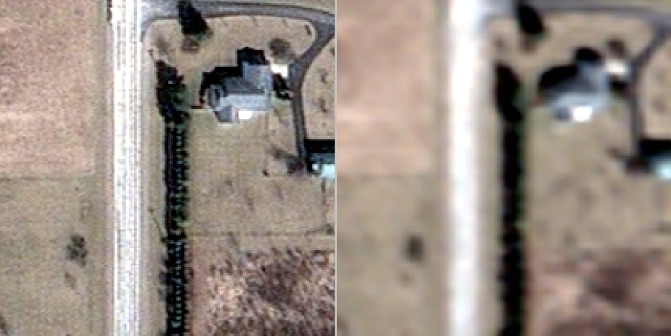
We used our Python package to evaluate the accuracy of our Super-Resolution processing block available on the UP42 marketplace. Below, you can review the pan sharpened image (ground truth) and model (the same model we used in the block) output image which super resolves the multispectral image to have the same resolution of pan sharpened image. Please note that we did the evaluation on the multispectral image, but the actual block will do superresolution on a pan sharpened image (For more information about this block, please have a look at this blog post and this paper).
 left: ground truth image; right: predicted image
We used the command to evaluate the two images as follows:
image-similarity-measures --org_img_path=path_to_first_img --pred_img_path=path_to_second_img --mode=tif --metric=ssimThe above command provides the SSIM value, but below you can find the values for all the metrics mentioned in this blog post for the above images.
- PSNR - 30.029
- SSIM - 0.77
- FSIM - 0.54
- ISSM - 0.17
- UIQ - 0.43
- SAM - 88.87
- SRE - 64.66
- RMSE - 0.03
In Closing
Image similarity detection is a hot topic in computer vision as it’s an essential component of many applications. There are various algorithms available to perform image similarity for different use cases. In this blog post, we introduced our new Python package that includes some of the common algorithms used for image similarity. We hope you find the Open Source package useful and welcome your feedback, ideas, and contributions directly to the project!


