Using TensorBoard while training land cover models with satellite imagery

Land cover classification is important for many applications, including disaster response, environmental monitoring, and remote monitoring. Land cover segmentation is an example where deep learning can be applied to extract valuable information from satellite images. In this blog post, I’ll run through some of the current challenges when training land cover segmentation models with high resolution satellite imagery and how to use TensorBoard to create a visual understanding of model training.

Satellite imagery classification using deep learning

The Data Science team at UP42 has been creating capacity around Deep Learning, especially applied for satellite imagery processing. We have already released a block in the marketplace that performs superresolution on SPOT and Pléiades imagery, achieving a final x4 increase in resolution. This block has been trained by the team and makes use of state of the art convolutional neural network architectures and using the UP42 platform to generate all the training data. We are additionally in the process of releasing a paper describing the research (Müller et al 2020).

The second project we are tackling revolves around land cover segmentation. Land cover classification or segmentation is the process of assigning each of the input imagery pixels a discrete land cover class (e.g. water, forest, urban, desert etc.). However, there are some challenges with achieving satisfactory segmentation results, especially when handling very high resolution imagery (e.g Pléiades). As one of the classic remote sensing problems, there are three main contributing factors to look at:

Scarcity of high-resolution training data

Most publicly available datasets are medium to low resolution (20m to 250m) and not suitable for training with 0.5m imagery. Available datasets are limited in geographical area and time scale.

Transferability of training datasets between sensors

Land cover models are often poor at generalizing. For example, a model trained with Sentinel-2 imagery in Senegal will produce poor results when classifying a Landsat image in Portugal.

Classification scheme differences based on geographic regions

Landscapes and because of this land cover, are extremely diverse across different geographies. As a result, different classification schemes are required to map out the diversity in an African city versus a rural American area.

Robinson et al. try to tackle these problems by making use of an adapted loss function that not only has the high resolution labeled data as input, but also an additional low resolution label data. This method showed promise in continental US where Robinson et al. was able to generate a satisfactory Land Cover Map using a model trained on a relatively small area in the North-East. We decided to build upon the work of Robinson et al. and have made contributions to the public repository.

Figure: Map showing the high-resolution labels generated by Robinson el at. consistency with NLCD (low resolution land cover dataset) over the entire US. Lower values represent an ‘inconsistency’ between the model prediction and the expected high resolution labels (using high-resolution label distributions per NLCD class from the Chesapeake Bay area). Areas for which there is no input data, or data errors prevented our model from running are shown in red (Robinson et al. 2019).

Visualizing model training

We are currently experimenting with different architectures based on the work of Robinson et al. to train a similar model in West Africa. During training, we felt that in order to debug the model performance and understand how we could improve it — we required a visual understanding for the imagery, labels and predictions. We had previously worked with TensorBoard, a TensorFlow visualization package, for drilling into metrics and decided to implement a visualization class for satellite imagery and labels used during training.

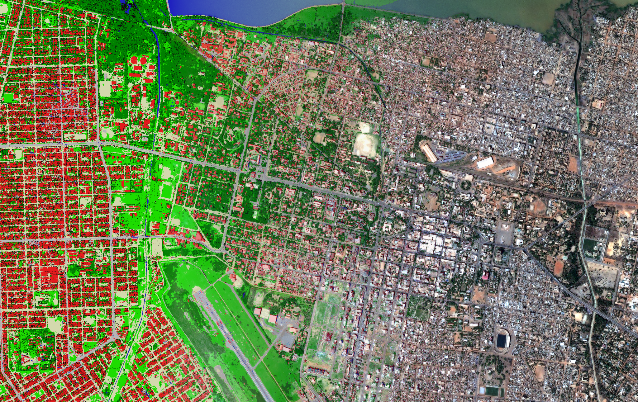
Above: SPOT imagery in Ouagadougou, Burkina Faso overlaid with Land Cover classes provided in Grippa & Georganos (2018).

How to implement TensorBoard

TensorBoard implementation is simple if you are using keras. Simply add an additional TensorBoard callback to your Model.fit call:

from tensorflow.keras.callbacks import TensorBoard

tensorboard_callback = tf.TensorBoard(logdir="logs")
model.fit(some_generator, callbacks=tensoboard_callback)

After running your model you can run the command below to visualize the logs results:

tensorboard --logdir=logs

If you save the logs folder in a GCP (Google Cloud Platform) bucket you can also serve the results directly from the bucket with:

gsutil cp -r logs gs://my-bucket/logs/
tensorboard --logdir=gs://my-bucket/logs/

In addition to being able to represent the metrics as scalars in TensorBoard you can also easily add imagery data in two different ways: by passing the imagery directly (as a tensor, or numpy array) or as a matplotlib figure converted into PNG with the tensorflow.summary.image method.

file_writer = tf.summary.create_file_writer("logs/")
with file_writer.as_default():
   tf.summary.image("train_label", some_batch)

Note that some_batch must be a numpy array of shape (batch, h,w, c). If c=1 then a grayscale image will be displayed. If values are of type float they will be clipped between 0-1. This expects RGB (Red, Green, Blue) or RGBA (Red, Green, Blue, Alpha) order of bands.

To use a matplotlib figure, use this method to convert to PNG (from the TensorBoard documentation):

def plot_to_image(figure):
   # Save the plot to a PNG in memory.
   buf = io.BytesIO()
   plt.savefig(buf, format="png")
   # Closing the figure prevents it from being displayed directly inside
   # the notebook.
   plt.close(figure)
   buf.seek(0)
   # Convert PNG buffer to TF image
   image = tf.image.decode_png(buf.getvalue(), channels=4)
   # Add the batch dimension
   image = tf.expand_dims(image, 0)
   return image
file_writer = tf.summary.create_file_writer("logs/")
with file_writer.as_default():
   tf.summary.image("train_figure",plot_image(some_matplotlib_fig))

In addition, TensorBoard gives you the chance to easily publish and share results of your experiments with tensorboard.dev. This is a free hosting service for TensorBoard that allows you to upload the dashboards you serve from your local machine with the commands below. Currently this service is still at a preview stage so only scalar dashboards are visible, but more will become available in the future. Note that these dashboards are fully public so make sure to not upload any sensitive information. To upload a dashboard to tensorboard.dev do:

tensorboard dev upload --logdir logs --name "My experiment"  --description "Simple display of training metrics"

If you run into issues please upgrade to the latest version of tensorboard with:

pip install -U tensorboard

A `ModelDiagnoser` class

In order to effectively use TensorBoard for diagnosing the land cover segmentation model we are working on, we built a custom callback that plots for every training epoch:

The source imagery, as an RGB composite;
The ground truth or labelled data, displayed with a custom color pallet;
The models prediction with the source imagery, with the same color pallet as the ground truth;
A confusion matrix of the predicted vs ground truth labels.

This solution was inspired by this StackOverflow answer. Here you can find the full implementation in our public repository. Below is a snippet of the on_epoch_end method:

def on_epoch_end(self, epoch, logs=None):
    def to_label(batch):
        label_batch = np.zeros(batch.shape[0:3])
        for i in range(batch.shape[0]):
            label_batch[i] = np.argmax(batch[i], axis=2)
        return label_batch

    output_generator = self.enqueuer.get()
    generator_output = next(output_generator)
    if self.superres:
        x_batch, y = generator_output
        y_batch_hr = y["outputs_hr"]
        y_batch_sr = y["outputs_sr"]
    else:
        x_batch, y_batch_hr = generator_output

    y_pred = self.model.predict(x_batch)
    if self.superres:
        y_pred, y_pred_sr = y_pred

    label_y_hr = to_label(y_batch_hr)
    label_y_pred = to_label(y_pred)

    with self.writer.as_default():
        for sample_index in [i for i in range(0, 3) if i <= self.batch_size - 1]:
            tf.summary.image(
                "Epoch-{}/{}/image".format(epoch, sample_index),
                x_batch[[sample_index], :, :, :3],
                step=epoch,
            )
            tf.summary.image(
                "Epoch-{}/{}/label".format(epoch, sample_index),
                self.plot_classification(
                    label_y_hr[sample_index], self.hr_classes_cmap,
                ),
                step=epoch,
            )
            tf.summary.image(
                "Epoch-{}/{}/pred".format(epoch, sample_index),
                self.plot_classification(
                    label_y_pred[sample_index], self.hr_classes_cmap,
                ),
                step=epoch,
            )
            tf.summary.image(
                f"Epoch-{epoch}/confusion_matrix",
                self.plot_confusion_matrix(
                    label_y_hr.squeeze(), label_y_pred.squeeze(),
                ),
                step=epoch,
            )

            if self.superres:
                tf.summary.image(
                    "Epoch-{}/{}/label_sr".format(epoch, sample_index),
                    self.plot_classification(
                        np.argmax(y_batch_sr[sample_index, :, :, :], axis=2),
                        self.sr_classes_cmap,
                    ),
                    step=epoch,
                )
                tf.summary.image(
                    "Epoch-{}/{}/pred_sr".format(epoch, sample_index),
                    self.plot_classification(
                        np.argmax(y_pred_sr[sample_index, :, :, :], axis=2),
                        self.hr_classes_cmap,
                    ),
                    step=epoch,
                )

In essence, the class defined here:

Inherits from the Callback class in keras, adding auxiliary variables as class arguments (such as the mapping of label to color);
Overwrites method on_epoch_end to write out the plots to tensorboard at the end of each epoch;
Overwrite the on_train_end method to close the file writer and the data generator.

In addition, three convenience methods are included for plotting:

plot_confusion_matrix - generates the confusion matrix plot with matplotlib by using the sklearn.metrics.confusion_matrix function;
plot_classification - generates a plot with matplotlib to get the appropriate color defined for each label;
plot_to_image - the function defined above to convert a matplotlib figure into a PNG for tensorflow.summary.image.

Image: Example of output in TensorBoard of ModelDiagnoser class.

Checkout this example dashboard uploaded to TensorBoard from one of the training runs we did with the Chesapeake Dataset.

Conclusion

Having a visualization component while training models with satellite imagery can be a great way to debug issues with model performance and/or training data. TensorBoard provides a simple way of creating a dashboard when training models with tensorflow and keras. With the ModelDiagnoser class you will be able to plug this into existing training workflows to get per epoch visualization of your model performance.

This has helped us understand, for example, that we needed further training data especially for the water class. In the future we intended to continue using TensorBoard in our model development, in tasks like object detection or instance segmentation.

Additional resources

If you want an excellent and extremely detailed look at tensorboard and all its possibilities have a look at this deep dive by Neptune.ai.

References

Ouagadougou very-high resolution land cover map (2018) https://doi.org/10.5281/zenodo.1290653

Müller, M., Ekhtiari, N., Almeida, R. M., Rieke, C., accepted for publication: Super-resolution of multispectral satellite images using convolutional neural networks. In: ISPRS Annals of the Photogrammetry, Remote Sensing and Spatial Information Sciences, preprint available at https://arxiv.org/abs/2002.00580

Robinson, C., Hou, L., Malkin, K., Soobitsky, R., Czawlytko, J., Dilkina, B.N., Jojic, N., 2019. Large Scale High-Resolution Land Cover Mapping With Multi-Resolution Data. 2019 IEEE/CVF Conference on Computer Vision and Pattern Recognition (CVPR) 12718–12727. https://doi.org/10.1109/CVPR.2019.01301

Rodrigo Almeida

Data Science Engineer

Tech