


After exploring the data platform from the two previous articles, we now turn our attention to the types of image processing you can do after you retrieve the data from UP42.
Ideally you can create a custom block, as described here.
For the sake of both brevity and simplicity, in this article, we'll delve into image analysis using the Orfeo Toolbox command line interface (OTB).
Our focus for this article is on basic image processing for remote sensing. Two recurring requests we receive from customers who are new to remote sensing are:
-
I obtained an analytic product and the RGB bands are not in the promised resolution.
-
I have pansharpened the analytic product but my image is too dark. How can I make it look better?
Developers who focus on geospatial imagery are just a subset of all developers, and if we restrict ourselves to satellite imagery and remote sensing, that set is even smaller. Our mission as a company is to democratize access to geospatial data of all kinds, which requires us to educate non-geospatial developers. Most developers are familiar with satellite imagery through the basemap (satellite) layer provided in popular mapping products, like HERE or Google maps. Those images are heavily processed by the map services to be visually pleasing and contain many diverse images stitched together, so that when you view it on the map, the image renders seamlessly as you move around.
One pitfall for using satellite imagery through products such as HERE or Google maps is that these are fixed in time, and it is not too clear when they were captured. Another pitfall is that the resolution of the images are often limited. Having access to the satellite imagery directly, as provided by UP42, allows you to set the desired date and to get the original satellite resolution. Additionally, the referencing of the image on the ground is the most precise possible, given that satellite providers have developed extensive networks of Ground Control Points (GCPs), combined with high-resolution terrain models that allow them to place a satellite image with high precision on the ground.
In the first article in this series, we explained how to order an image. In the notebook associated with it, we ordered a Display product. Display products offer the best-looking image possible, from a human visual perception perspective. They are generated via a color space transformation that is dependent on the position of the pixel on the image: tone mapping.
However, the type of image most frequently requested by our customers is called Analytic. It has no tone mapping and is supposed to represent a correct assessment of the radiated energy by the area being imaged. It allows you to do all manners of analysis on the data, e.g., vegetation, water, fire, etc. In this article we explain how to:
-
Process the image, so that the RGB bands are set to the maximum resolution.
-
Create a visually pleasing image from the image previously obtained.
Visually pleasing here means fit to be viewed by humans. But as we will see, what we obtain in the end, although is a big improvement from the original Analytic product, it is inferior to the corresponding Display product. Our goal here is not to provide a shortcut to avoid ordering a Display product if you need the best possible visually pleasing image, but rather to explore basic image processing for remote sensing and gain awareness to the specificity of remote sensing images in general and satellite imagery in particular.
Pansharpening in a nutshell
Introduction
Image sensors behave quite differently from the human eye. They do not have color specific sensors like we have. Image sensors view the objects in the world such that all light wavelengths are treated equally, for the most part. Of course there are specialized sensors, e.g., for infrared bands, ultraviolet etc, but if we concern ourselves only with common usage photography, the sensors view the world as a continuous range of gray tones. Humans have a limited ability to distinguish shades of gray. We have specialized sensors in our eye that distinguish Red, Green and Blue colors (RGB).
Since sensors see the world in gray, to create an RGB signal, filters need to be applied so that only the relevant part of the light spectrum is captured. This is usually done through Bayer filters. At minimum, it takes four (4) pixels from the sensor to create an RGB equivalent pixel. Since the resolution is defined for the gray level image, if the resolution is 50 cm, i.e., a pixel represents a 50x50 cm object on the ground, then an RGB pixel would be 1/4 of this, i.e., 2 m. This is exactly what the Pléaides satellite constellation provides.
The question is: can we have the high-resolution gray level band, otherwise termed the panchromatic band, somehow bring that band information to bear on the RGB images, such that they get upgraded to 50 cm resolution? The answer is yes and this process is called Pansharpening or resolution merging.
It is well beyond the scope of this article to delve into the details of Pansharpening, instead we are going to rely on the excellent algorithm for Pansharpening which is available in the Orfeo Toolbox utility BundleToPerfectSensor.
Of course we could have used the pansharpening processing block available in the UP42 marketplace. But remember that we want to explore the utilities in Orfeo Toolbox and also understand what is happening to the image as we process it, hence we will do it ourselves.
Pansharpening with the Orfeo Toolbox
Pansharpening in Orfeo Toolbox is usually done through the BundleToPerfectSensor utility. It combines two actions into one:
-
Upsampling of the multispectral bands (RGB, NIR, etc., denoted XS) to the resolution of the panchromatic band (PAN). This is done through the SuperImpose utility. The upsampling is done by interpolation.
-
Fusion/merging of the data from PAN with XS. This is done via the Pansharpening utility.
The default method for fusion is called Ratio Component Substitution (RCS). It is described in the OTB User Guide. The panchromatic band can be seen as an extension of a spectral band to higher wave numbers, i.e., the multispectral bands can be obtained through low pass filtering of the panchromatic band. Doing this for each band generates the pansharpened data.
Example
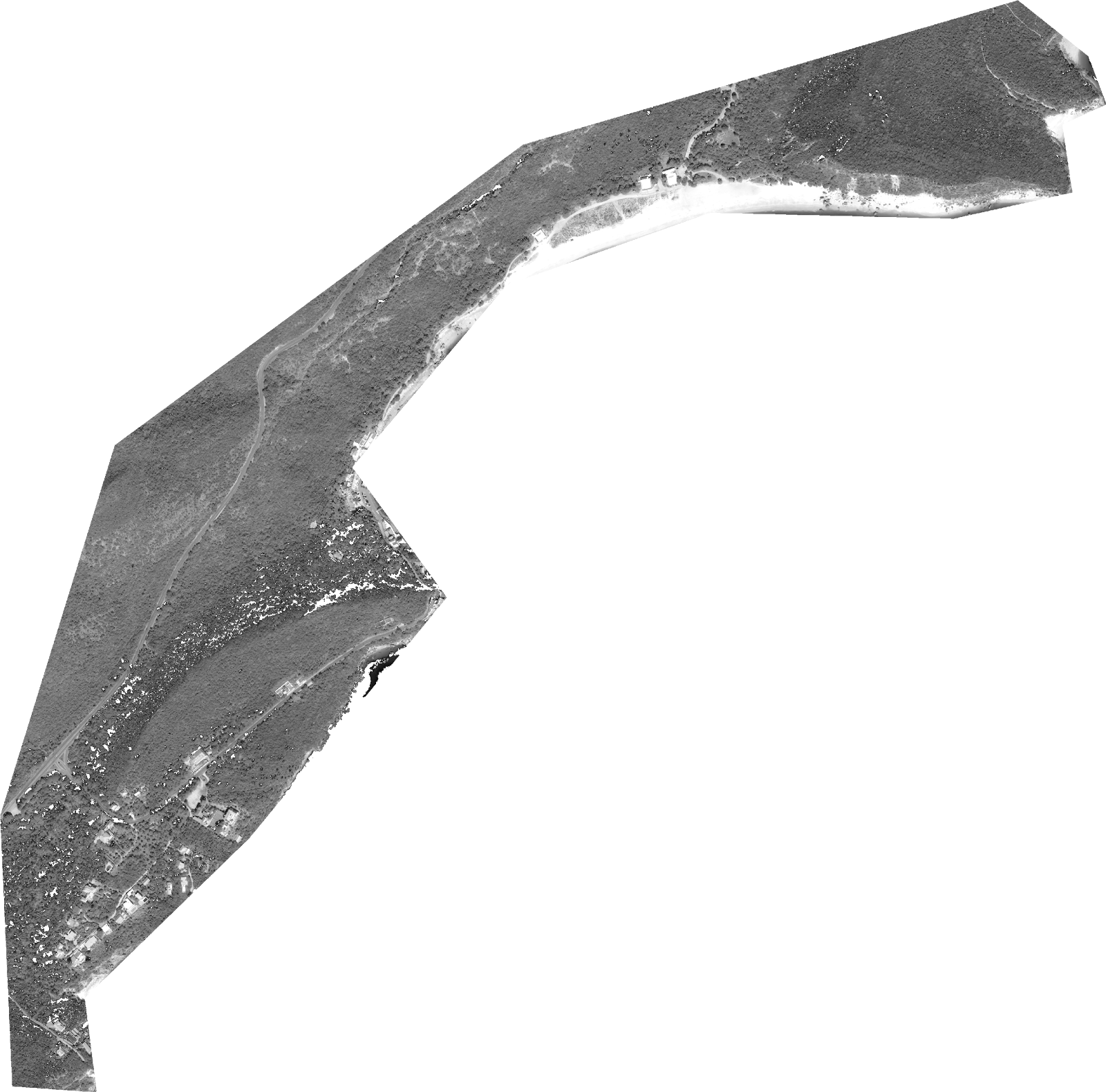
We are going to consider the AOI we used for the data ordering 101 notebook. Here we ordered an Analytic product, i.e, an orthorectified, atmospherically corrected version of the image, delivered as a 16 bit GeoTIFF.
Issuing the command:
otbcli_DynamicConvert -type.linear.gamma 2.2 -channels rgb \
-in arrabida_pansharpened.tif \
-out arrabida_pansharpened_gamma22.tif \
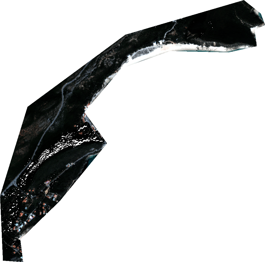
-ram 512generates the pansharpened image.
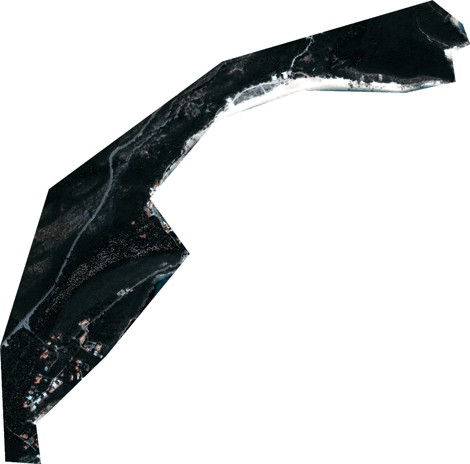
As we can see, we cannot use this image to visually display this AOI. It looks toO dark to us. This comes from the fact that the tone distribution is uniform, while human vision uses non-uniform distribution (logarithmic).
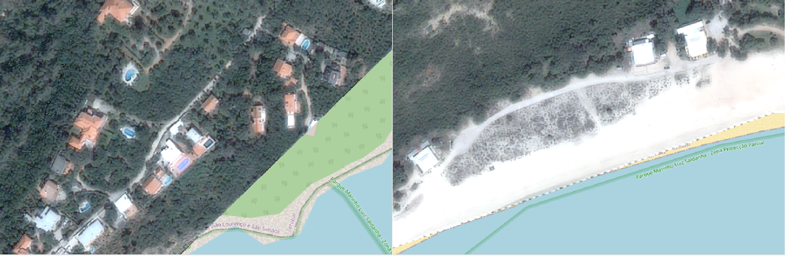
Let us compare the pansharpened image with the corresponding visual product.
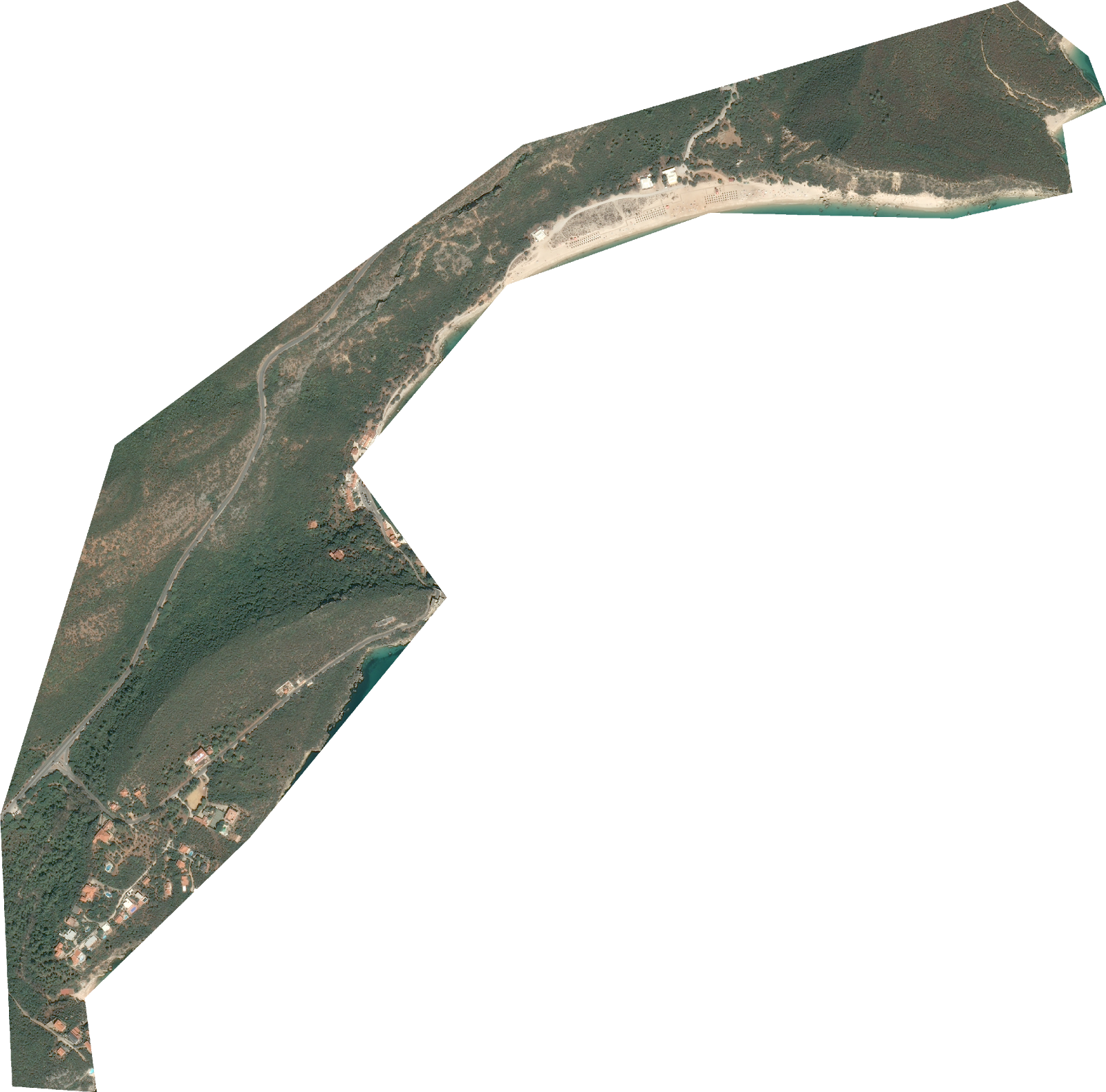
We now can see details that we could not see before. Let's zoom in on a specific area.
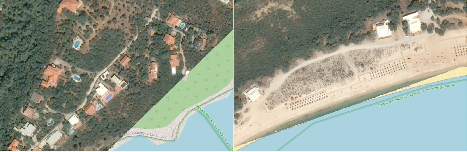
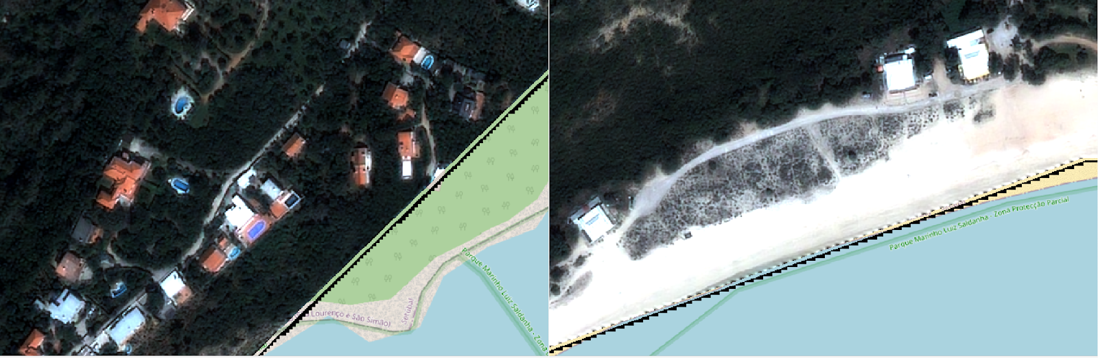
Of course, we are comparing different things. The pansharpened image function is not to be visually pleasing, but rather to be precise, i.e., as close to the values captured by the satellite camera as possible, after atmospheric correction (and pansharpening).
The question then is: can we create visually pleasing images using an analytic product as the source? If yes, then how does it compare to the visual product?
We attempt to answer these two questions below. In the process we hope to gain a deeper understanding of remote sensing images and the challenges they pose to image processing.
Creating visually pleasing images in a nutshell
Introduction
Now that we have a full resolution RGB image how can we make it visually pleasing? Although we have set the RGB image to the full resolution, if we look at the image, it appears dark and most features are hard to distinguish for the human eye. This is to be expected since we imported the linear response from the panchromatic (gray level) band into the RGB bands. The human eye doesn't respond linearly to light, but logarithmically instead. So what we need to do is to transform the color space in the RGB image so that the histogram is adapted to the human eye. OTB has an utility precisely for that called DynamicConvert.
This utility rescales the input image and also applies a gamma correction, if specified.
Rescaling and gamma correction
The rescaling needs to be done because the original image (the pansharpened image) is a 32 bit image where the pixel values are real numbers, while the visually pleasing image we want is a 8 bit image where the pixel values are integers from 0 up to 255. You can confirm that using the OTB utility ReadImageInfo.
When we rescale we can not only do a simple scaling, but we can also do a mapping of the values using an exponential law.
where is the output multispectral image pixel triple values (RGB) and is the input multispectral image pixel values. is a constant.
This is called gamma correction. Usually this has two components: an encoding part, where , termed gamma compression, and a decoding part, where , termed gamma expansion. The encoding part is done to save space, since we are subsetting the full set of values.
This is used in not only digital cameras, but also in computer displays and other imaging devices: whenever there is the need to transform the linear response of an imaging device into non-linear, such that humans can better perceive it. For example, a digital camera corrects the sensor linear response by doing gamma compression, saving space, and when that image is viewed in a computer monitor, gamma expansion is done, so that the full tonal range is properly displayed.
Of course there is no gamma compression in satellite imagery. You always get the full dynamic range. But we can reason by analogy and take advantage of the non-linear brightening effect of gamma expansion to enhance the image.
The exact value will depend on the specific image. In this case we ended up with a value . You should always experiment with multiple values to find out which one gives the best result.
Issuing the command:
otbcli_DynamicConvert -type.linear.gamma 2.2 -channels rgb \\
 -in arrabida_pansharpened.tif \\
 -out arrabida_pansharpened_gamma22.tif \\
 -ram 512
Why just not use histogram equalization?
Introduction
Histogram equalization is commonly used to increase the contrast in images with a large dynamic range. It is equivalent to applying a low pass filter since it homogenizes the pixel values and therefore inevitably destroys finer details of the image specially if those details are distributed throughout the image.
Orfeo Toolbox has an utility precisely for that.
Remote sensing images are for the most part very rich in fine details, the higher the resolution the greater the possibility of having very fine details distributed throughout the image.
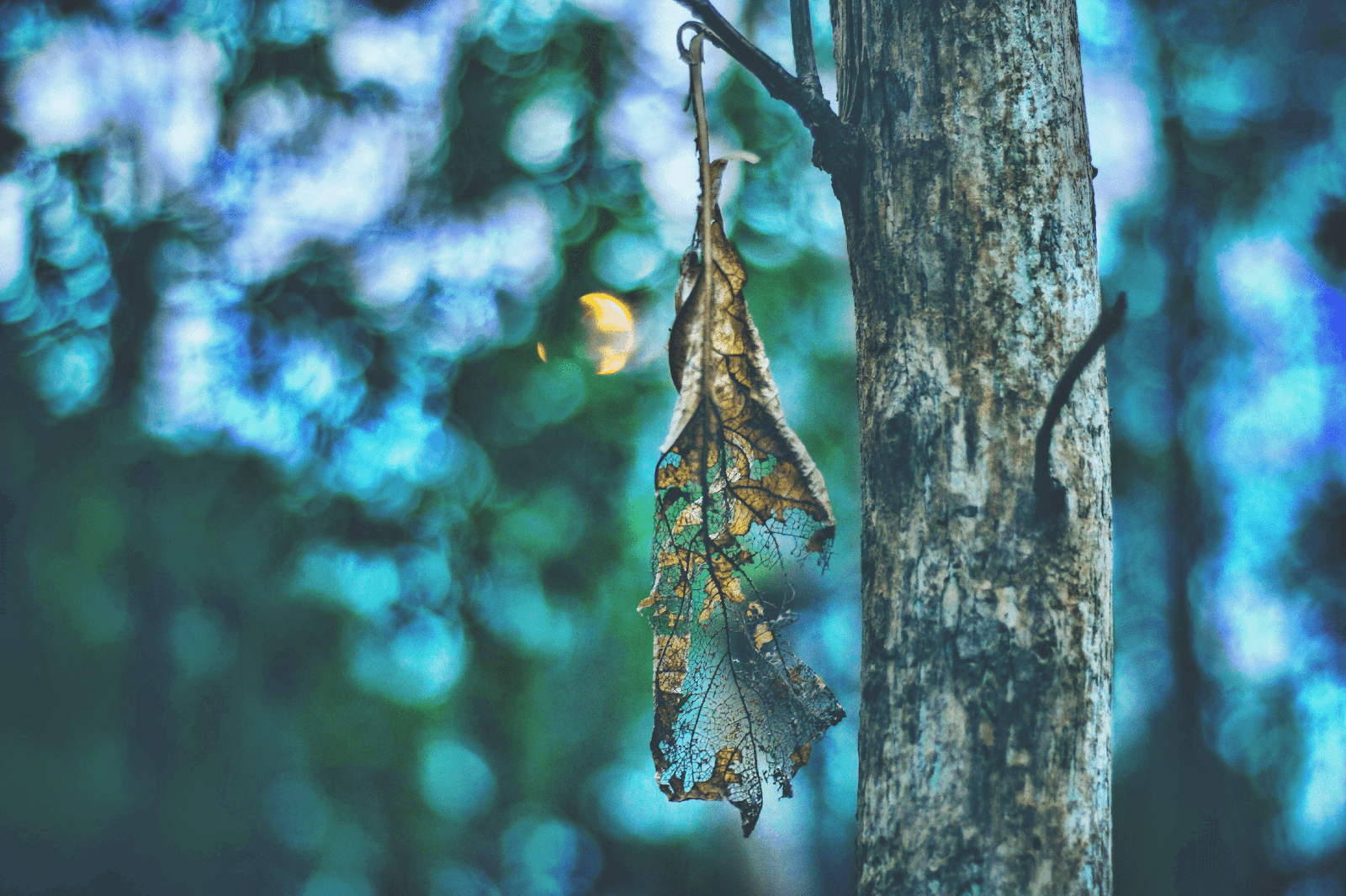
Histogram equalization works well if the image has a clear subject and the remainder is just the image foreground. To illustrate this, let us look at a low contrast image from Unsplash:

We can see that the focused tree and dry leaf is hard to distinguish from the unfocused foreground.
Now if we use ContrastEnhancement from the Orfeo Toolbox, using a local luminance mode with a contrast limiting factor of 4:
otbcli_ContrastEnhancement -in <infile> -out <outfile> -mode lum -hfact 4where infile is the input file name and outfile is the output file name.
We obtain the much clearer image below:
Applying histogram equalization to our image
Let us apply histogram equalization to our image using the same settings as above for the leaf and tree trunk image. In fact, by default a localized approach is used. I.e., Orfeo Toolbox implements Adaptive Histogram Equalization with contrast limit. In each region of a given size, the histogram is equalized and, to suppress noise amplification, the contrast is limited. Let us use a 256x256 window for histogram equalization.
  otbcli_ContrastEnhancement -in arrabida_pansharpened.tif\
-out arrabida_pansharpened_enhanced_w256.tif \\
 -mode lum \\
 -hfact 4 \\
 -spatial.local.w 256 \\
 -spatial.local.h 256
This is equivalent to:
otbcli_ContrastEnhancement -in arrabida_pansharpened.tif\
-out arrabida_pansharpened_enhanced_w256.tif \\
 -mode lum \\
 -hfact 4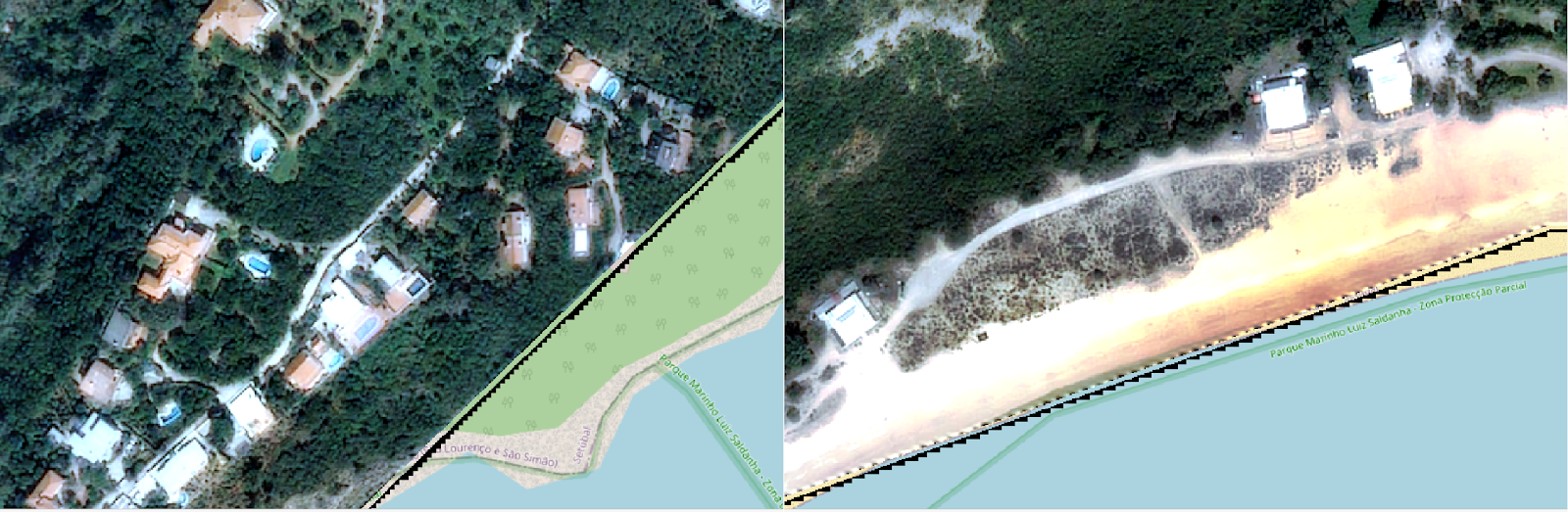
We continue to have artifacts in the image and loss of detail. We could try other value combinations, but this doesn't look like a promising path, if we compare it with what we obtained using gamma correction above. In the end simplicity wins.
Lookup table approach
Although not applicable to all imagery providers, Airbus provides as metadata a XML file that contains a lookup table to map the values in the image to a visually pleasing image. In this case the file is named LUT_PHR1B_MS_202203181124065_ORT_4382a229-3ef9-42f5-c293-f2f498a92140-001.XML.
The format of the lookup table is the one supported by MapServer. So by iterating through all the bands we would do a simple replacement of values and thus get a visually pleasing image. However, since we pansharpened the image there are new pixel values–from the bicubic interpolation when we upsampled the multispectral bands–and therefore we cannot use the lookup table as it is. If we had obtained an already pansharpened image, then the lookup table would be adjusted to that and we could then use it. As it stands, it is of limited use, unless you don't want to pansharpen the image.
Conclusions
Remote sensing images pose significant challenges to be processed. What would work well in simpler images doesn't perform as well for satellite imagery. Great care needs to be taken so that details are not lost when the image is processed. Simpler processing methods, like gamma correction, should be used before any other more elaborate methods, since these tend to introduce more artifacts in the image.
We have barely scratched the surface. There is much more to be explored. Here, we just experimented with obtaining visually pleasing images from analytic products.
It is also clear that obtaining the display product is the way to go if you want the best possible looking image. Therefore the expedient we used above should not be used if, for example, you want to apply a classification algorithm based on neural networks. The latter is very sensitive to artifacts and it will create a lower quality model if you are training it or provide lower quality inference results in a previously trained model.
Image credits
Analog camera and film rolls photo by Dicky Jiang on Unsplash.
Tree trunk with leaf photo by Amritanshu Sikdar on Unsplash.


